Construct a custom fit for an extension of the MRP: a double-Schechter function.

Note: this example is almost identical to that found in the R package ``tggd`` in the ``tggd_log`` documentation.

While mrpy has several in-built routines which aid in fitting the MRP function to data, it does not natively support fitting extensions of the MRP, such as double-Schechter functions. For such functions, one can fairly simply create custom fits using the methods found in Scipy, for example.

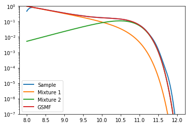
In this example, we create a double-Schechter galaxy stellar mass function (GSMF) down to a target stellar mass (xmin) of log10(SM) = 8. We use data from Baldry+2012 to define the function:

Both mixtures have

\[ \begin{align}\begin{aligned}M_\star \equiv \log_{10} \mathcal{H}_\star = 10.66\\and\end{aligned}\end{align} \]

\[\beta = 1\]

Mixture 1 has:

\[\alpha_1 = -1.47\]

\[\phi^\star_1 = 0.79\times 10^{-3}\]

Mixture 2 has:

\[\alpha_2 = -0.35\]

\[\phi^\star_2 = 3.96\times 10^{-3}\]

Furthermore, we use only the purely statistical routines of mrpy to achieve our results:

# Imports
%matplotlib inline
import matplotlib.pyplot as plt
import numpy as np
from scipy.stats import gaussian_kde
from scipy.optimize import minimize

from mrpy.base import stats

First we define objects which capture the statistical quantities of each mixture:

mix1 = stats.TGGDlog(10.66,-1.47,1.0,8)
mix2 = stats.TGGDlog(10.66,-0.35,1.0,8)

\(\phi^\star\) is defined as the value of the pdf in log-space at the pivot scale by \(e\), i.e.

\[\phi^\star = PDF(M_\star)\times \frac{e}{\ln(10)}\]

This normalisation is important in our sampling since it gives the ratio of samples produced by each mixture. We can produce the relevant normalisation using:

M1norm=0.79/mix1.pdf(10.66)
M2norm=3.96/mix2.pdf(10.66)
Mtot=M1norm+M2norm

Now say we would like to sample 1e5 galaxies, we can produce these like so:

Nsamp=1e5

np.random.seed(100)

mix1_sample = mix1.rvs(int(Nsamp*M1norm/Mtot))
mix2_sample = mix2.rvs(int(Nsamp*M2norm/Mtot))

gal_sample = np.concatenate((mix1_sample,mix2_sample))

Let’s plot the distribution we’ve just created, to check if everything has worked okay:

# Create x array to plot against
x = np.linspace(8,12,401)

plt.plot(x,gaussian_kde(gal_sample)(x),label="Sample", lw=2)

plt.plot(x,mix1.pdf(x) * M1norm/Mtot,label="Mixture 1", lw=2)
plt.plot(x,mix2.pdf(x) * M2norm/Mtot,label="Mixture 2", lw=2)
plt.plot(x,mix1.pdf(x) * M1norm/Mtot + mix2.pdf(x) * M2norm/Mtot, label="GSMF", lw=2)
plt.yscale('log')
plt.ylim((1e-7,1))
plt.legend(loc=0)

<matplotlib.legend.Legend at 0x7fa87a9d5210>

Now we can try to fit the mixed model. The trick here is we fit for the mixture using an additional parameter \(\lambda\), where one component is multiplied by \(\lambda\) and the other \(1-\lambda\). We define it so that M1norm/Mtot=lambda and M1norm/Mtot=1-lambda. Here’s our model:

def mix_lnl(par,data):
    mix1 = stats.TGGDlog(par[0],par[1],1.0,8)
    mix2 = stats.TGGDlog(par[0],par[2],1.0,8)

    return -np.sum(np.log(mix1.pdf(data)*par[3] + mix2.pdf(data)*(1-par[3])))

Now we can perform the fit, using a downhill-gradient method of our choice. The fit is probably not fantastic though. Generalised Gamma distributions (including truncated ones) display poor convergence properties using ML. Full MCMC is a better route when trying to fit GSMF type data. And the data certainly should not be binned!

GSMFfit = minimize(mix_lnl, x0=[10,-2,0,0.5], args=(gal_sample,), bounds=[(9,12),(-2.5,-0.5),(-1.0,0.5),(0.0,1.0)])

print "Maximum likelihood parameters: ", GSMFfit.x

Maximum likelihood parameters:  [ 10.65427592  -1.46844631  -0.34935003   0.83445411]

This accords very well with our input parameters!