How to get started
This series of examples shows the very basics of how to get started with MRPY, using the different functionality. These examples aren’t “real world” ones, just toy ones to show the basic idea.
In [1]:
# General Imports
%matplotlib inline
import matplotlib.pyplot as plt
import numpy as np
Core Functionality
Core functionality (i.e. calculation of the MRP function given input
parameters, plus some other functions useful for normalising) is in the
core module:
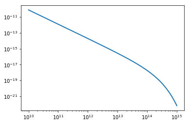
In [2]:
from mrpy import dndm      # resides in the base.core module, but imported into top-level namespace
m = np.logspace(10,15,500) # Create an array of masses
dn = dndm(m, logHs=14.0, alpha=-1.8, beta=0.85) # Create the MRP mass function
plt.plot(m,dn,lw=2)
plt.xscale('log')
plt.yscale('log')
Pure Stats
If you don’t care so much about the fact that the MRP is good for halo
mass functions (or don’t know what a halo mass function is…), but want
to use the statistical distribution, you’ll want the stats module.
It contains an object called TGGD (short for Truncated Generalised
Gamma Distribution), which has many statistical quantities and methods
available (such as producing random variates, mean, mode etc.)
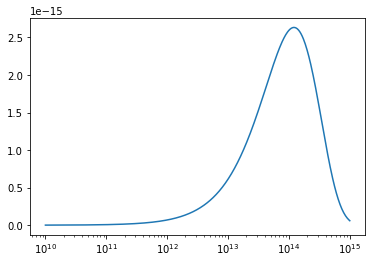
In [3]:
from mrpy import TGGD
tggd = TGGD(scale=1e14,a=1.0,b=0.85,xmin=1e10)
print "Mean: ", tggd.mean  # Mean of the distribution
print "Mode: ", tggd.mode  # Mode of the distirbution
print "Variance: ", tggd.variance # Variance of the distribution
print "Mean of sample: ", np.mean(tggd.rvs(1e5))  #Produce 1e5 random variates and take the mean
plt.plot(m, tggd.pdf(m))      #Plot the PDF
plt.xscale('log')
Mean:  2.84867015869e+14
Mode:  1.21070004341e+14
Variance:  4.79705281452e+28
Mean of sample:  2.83287193279e+14
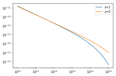
Physical Dependence
The physical_dependence module contains a counterpart to the basic
dndm function, called mrp_b13, which returns the best-fit MRP
according to input physical variables (redshift, matter density, rms
mass variance). These are derived from fits to the theoretical mass
function of Behroozi+2013.
In [4]:
from mrpy import mrp_b13
dndm_z1 = mrp_b13(m,z=1)           # HMF at redshift 1
dndm_z0 = mrp_b13(m,sigma_8=0.85)  # HMF at redshift 0 but sigma_8=0.85
plt.plot(m,dndm_z1,label="z=1")
plt.plot(m,dndm_z0,label="z=0")
plt.legend(loc=0)
plt.xscale('log')
plt.yscale('log')
Fitting MRP
Fitting Curve Data
The fit_curve module contains routines to fit the MRP to
binned/curve data. This can be a theoretical curve, or binned halos (or
other variates). There are several options available, and the gradient
of the objective function is specified analytically to improve
performance. See Murray, Robotham, Power, 2016 (in prep.) for more
details.
In [5]:
from mrpy.fitting.fit_curve import get_fit_curve
dn = dndm(m,logHs=14.0,alpha=-1.9,beta=0.75,norm=1)
result, curve_obj = get_fit_curve(m,dn,[14.5, -1.8, 0.85,0.],
                                  bounds = [[None,None], [-2,-1.5], [0.2,1.5], [None,None]]) #The bounds argument is very important at this stage.
print result
plt.plot(curve_obj.logm,curve_obj.dndm()/dn-1,lw=2)
      fun: 1.6704623362075916e-12
 hess_inv: <4x4 LbfgsInvHessProduct with dtype=float64>
      jac: array([ -8.60315661e-05,  -1.13296916e-04,   6.03274702e-05,
        -3.79420248e-06])
  message: 'CONVERGENCE: REL_REDUCTION_OF_F_<=_FACTR*EPSMCH'
     nfev: 28
      nit: 25
   status: 0
  success: True
        x: array([  1.40000001e+01,  -1.90000003e+00,   7.50000058e-01,
        -5.62234817e-07])
Out[5]:
[<matplotlib.lines.Line2D at 0x7f072e383dd0>]
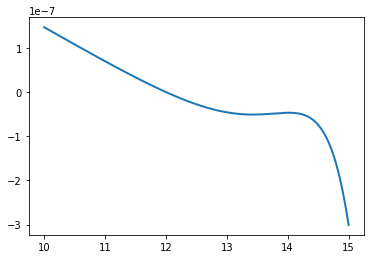
In the previous example, we simply fit the four MRP parameters to the input curve. Options can be specified to constrain the normalisation via the known mean density of the Universe (see MRP, 2017 Appendix C.1 for details).
Fitting Samples
To fit actual samples of halos, use the fit_sample module. At this
stage, only samples with no measurement uncertainties, and a constant
volume (per subsample) are supported. Usefully, this covers the case of
output halos from simulations. Within this context, either a
downhill-gradient method or MCMC can be used.
We hope to provide more general fitting scenarios via configuration with other packages in the future.
An example of using the downhill method is as follows:
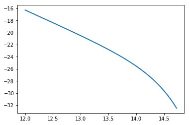
In [6]:
from mrpy.base.stats import TGGD
from mrpy.fitting.fit_sample import SimFit

# Create some mock data to fit
r = TGGD(scale=1e14,a=-1.8,b=1.0,xmin=1e12).rvs(1e5)
r = np.sort(r)

# Create fit object, specifying parameter bounds
fitobj = SimFit(r,hs_bounds=(12,16),alpha_bounds=(-1.99,-1.6),beta_bounds=(0.5,1.5))

# Run downhill gradient method
res, obj = fitobj.run_downhill()

# Print the resulting parameters
print "Resulting Parameters: ", res.x

# The "obj" returned is a list of PerObjLike objects defined at the result, containing lots of methods and quantities:
print "Hessian at solution: ", obj[0].hessian
print "Covariance at solution: ", obj[0].cov

# Plot the mass function from obj (the logm contains all the masses from the fit)
plt.plot(obj[0].logm,obj[0].dndm(log=True),lw=2)
Resulting Parameters:  [ 13.9900839   -1.79700413   0.94765685 -24.43903982]
Hessian at solution:  [[-1838656.7724181   1485394.57073756  -508029.87769594  -427802.81517913]
 [ 1485394.57073756 -1328344.72287371   412360.36967558   351970.2695528 ]
 [ -508029.87769594   412360.36967558  -142628.15625157  -118826.3858363 ]
 [ -427802.81517913   351970.2695528   -118826.3858363   -100000.08553355]]
Covariance at solution:  [[ 0.00077558 -0.00025638  0.00122131 -0.00567158]
 [-0.00025638  0.00010004 -0.00046645  0.00200319]
 [ 0.00122131 -0.00046645  0.00287933 -0.01028797]
 [-0.00567158  0.00200319 -0.01028797  0.04354857]]
Out[6]:
[<matplotlib.lines.Line2D at 0x7f072cbebd50>]